# Load and prep data

library(tidyverse)
theme_set(theme_minimal())

library(readxl)
scooby <- read_excel("_internal/scooby.xlsx")

scooby_sm <- scooby |>
  filter(format == "TV Series") |>
  select(title,
         date_aired,
         imdb,
motive) Working with factors in R
forcats
R-bloggers
Need to change the ordering of a categorical variable? Update its labels? Create an ‘other’ category? You’ve come to the right place.
Categorical variables (or factors as they are referred to when working in R) are variables that assign observations to specific groups. This post will cover some of the most common problems you may encounter while trying to visualize or model such variables.
Throughout, I’ll refer to the scooby data set, originally sourced from kaggle but modified slightly for use in my vids and in this post. A download link can be found at the end of this tutorial.
Factor, character, and other vector types
As a general rule, tidyverse functions treat character vectors as factors. For instance, we can apply dplyr::count to scooby$motive, even though the latter just consists of strings.
glimpse(scooby_sm)Rows: 374
Columns: 4
$ title <chr> "What a Night for a Knight", "A Clue for Scooby Doo", "Hass…
$ date_aired <dttm> 1969-09-13, 1969-09-20, 1969-09-27, 1969-10-04, 1969-10-11…
$ imdb <dbl> 8.1, 8.1, 8.0, 7.8, 7.5, 8.4, 7.6, 8.2, 8.1, 8.0, 8.5, 8.2,…
$ motive <chr> "Theft", "Theft", "Treasure", "Natural Resource", "Competit…scooby_sm |>
count(motive)# A tibble: 17 × 2
motive n
<chr> <int>
1 Abduction 3
2 Assistance 2
3 Competition 130
4 Conquer 33
5 Counterfeit 6
6 Entertainment 3
7 Extortion 3
8 Imagination 1
9 Inheritance 6
10 Natural Resource 19
11 Preservation 10
12 Safety 2
13 Simulation 2
14 Smuggling 19
15 Theft 93
16 Treasure 40
17 <NA> 2Use as.factor() to explicitly coerce variables to factors. This is particularly useful when category levels are numeric, like am (automatic/manual transmission) in the built-in mtcars set, since functions like ggplot will otherwise attempt to treat them as continuous variables. For instance, we can’t get directly get a side-by-side boxplot of mpg vs am.
glimpse(mtcars)Rows: 32
Columns: 11
$ mpg <dbl> 21.0, 21.0, 22.8, 21.4, 18.7, 18.1, 14.3, 24.4, 22.8, 19.2, 17.8,…
$ cyl <dbl> 6, 6, 4, 6, 8, 6, 8, 4, 4, 6, 6, 8, 8, 8, 8, 8, 8, 4, 4, 4, 4, 8,…
$ disp <dbl> 160.0, 160.0, 108.0, 258.0, 360.0, 225.0, 360.0, 146.7, 140.8, 16…
$ hp <dbl> 110, 110, 93, 110, 175, 105, 245, 62, 95, 123, 123, 180, 180, 180…
$ drat <dbl> 3.90, 3.90, 3.85, 3.08, 3.15, 2.76, 3.21, 3.69, 3.92, 3.92, 3.92,…
$ wt <dbl> 2.620, 2.875, 2.320, 3.215, 3.440, 3.460, 3.570, 3.190, 3.150, 3.…
$ qsec <dbl> 16.46, 17.02, 18.61, 19.44, 17.02, 20.22, 15.84, 20.00, 22.90, 18…
$ vs <dbl> 0, 0, 1, 1, 0, 1, 0, 1, 1, 1, 1, 0, 0, 0, 0, 0, 0, 1, 1, 1, 1, 0,…
$ am <dbl> 1, 1, 1, 0, 0, 0, 0, 0, 0, 0, 0, 0, 0, 0, 0, 0, 0, 1, 1, 1, 0, 0,…
$ gear <dbl> 4, 4, 4, 3, 3, 3, 3, 4, 4, 4, 4, 3, 3, 3, 3, 3, 3, 4, 4, 4, 3, 3,…
$ carb <dbl> 4, 4, 1, 1, 2, 1, 4, 2, 2, 4, 4, 3, 3, 3, 4, 4, 4, 1, 2, 1, 1, 2,…ggplot(mtcars, aes(x = am,
y = mpg)) +
geom_boxplot() # not what we wantWarning: Orientation is not uniquely specified when both the x and y aesthetics are
continuous. Picking default orientation 'x'.Warning: Continuous x aesthetic
ℹ did you forget `aes(group = ...)`?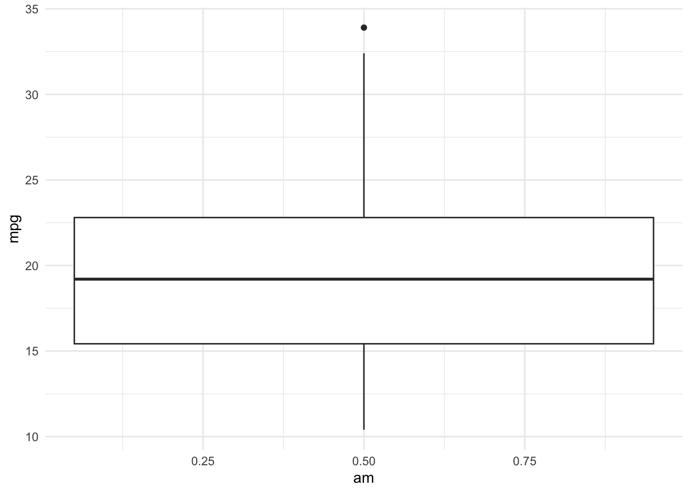
While it’s fine to follow the recommendation given in this warning message, it may be better to just convert am to a factor once and for all:
mtcars2 <- mtcars |>
  mutate(am = as.factor(am))

ggplot(mtcars2, aes(x = am,
                    y = mpg)) +
  geom_boxplot()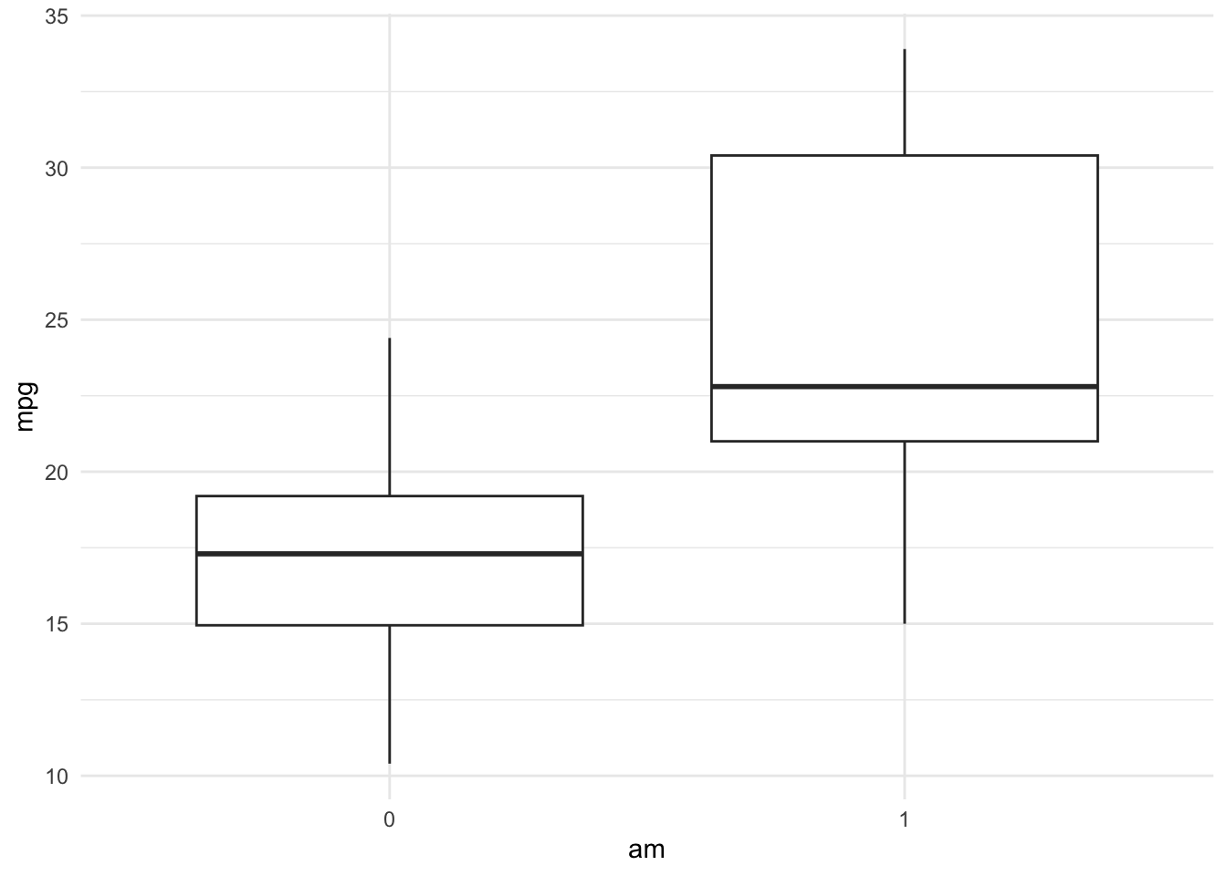
Relabeling factors
There are many options for changing the text used to label factor levels, but fct_recode() is a solid choice.
mtcars2 <- mtcars2 |>
  mutate(am = fct_recode(am,
                         "automatic" = "0",
                         "manual" = "1"))
mtcars2 |>
  count(am)
am n
1 automatic 19
2 manual 13Notice the syntax, “new_name” = “old_name”, which is common in tidyverse R.
When you have a large number of different factor levels, it may be helpful to lump the less common ones into an “other” category. For instance, the next chunk combines all categories with fewer than 20 occurrences.
scooby_sm2 <- scooby_sm |>
  mutate(motive = fct_lump_min(motive,
                               min = 20))
scooby_sm2 |>
  count(motive) |>
  arrange(-n)
# A tibble: 6 × 2
motive n
<fct> <int>
1 Competition 130
2 Theft 93
3 Other 76
4 Treasure 40
5 Conquer 33
6 <NA> 2Also check out fct_lump_n() to specify the number of levels retained, fct_lump_prop() to lump low-percentage levels, and fct_lump_lowfreq() to try to force the new “Other” level to have lowest frequency.
Rearranging levels
Sometimes the order of factor levels matters, for instance in a bar chart. The default odering is alphanumeric.
ggplot(scooby_sm2,
       aes(x = motive)) +
  geom_bar()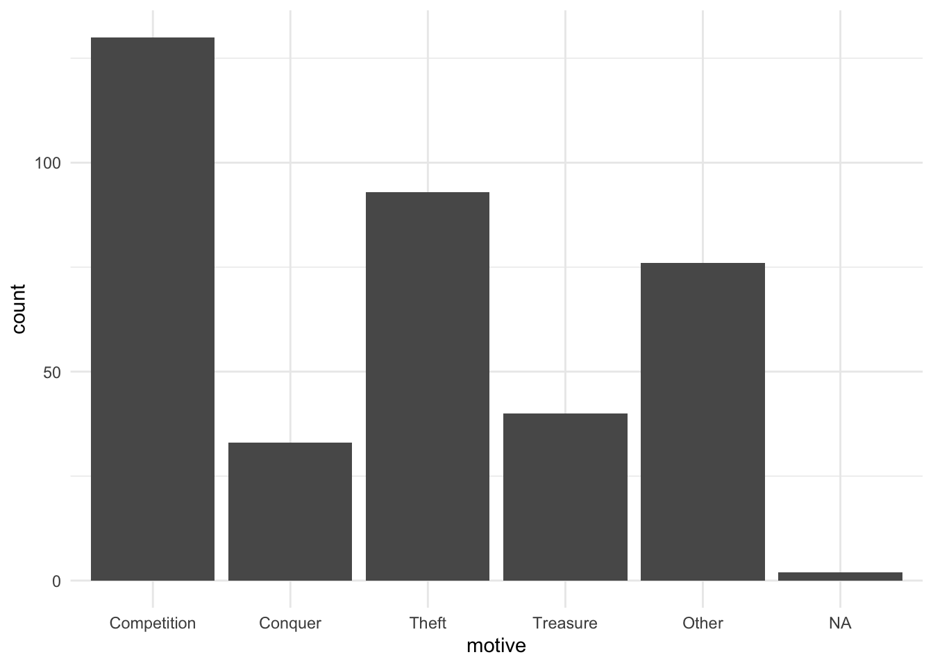
Use fct_relevel() to shift levels to the front. For instance, the next code chunk places the motives Treasure and Theft before Compitition and others.
scooby_sm3 <- scooby_sm2 |>
  mutate(motive = fct_relevel(motive,
                              "Treasure",
                              "Theft"))

ggplot(scooby_sm3,
       aes(x = motive)) +
  geom_bar()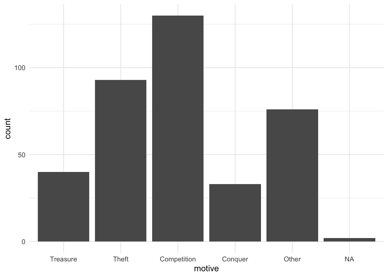
Often, you just want to put the most common factor levels first. Use fct_infreq() to accomplish this.
ggplot(scooby_sm2, aes(x = fct_infreq(motive))) +
  geom_bar()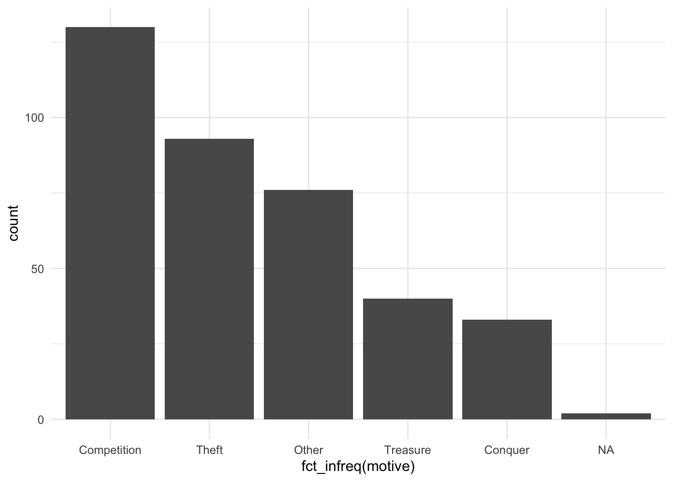
You can also reverse the order of the factor levels with fct_rev.
Reordering levels using a second variable
For some plots, it can be natural to order a categorical variable using a numeric one. For instance, in the next plot, it would be preferable to show the various motives in increasing order of imdb ratings.
ggplot(scooby_sm3, aes(x = motive,
                       y = imdb)) +
  geom_boxplot()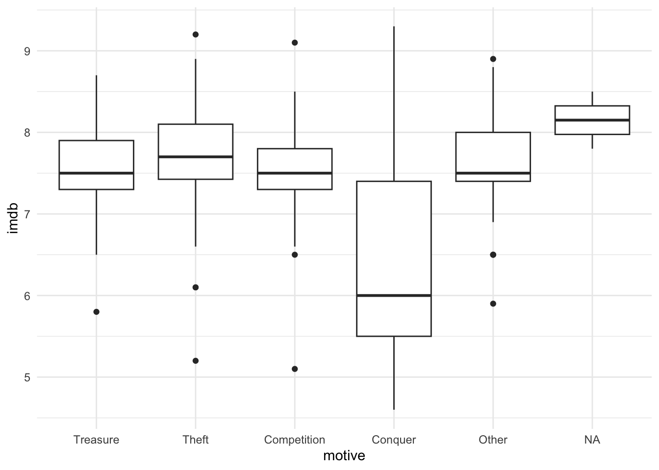
Use fct_reorder to accomplish this.
scooby_sm4 <- scooby_sm3 |>
  mutate(motive = fct_reorder(motive,
                              imdb))

ggplot(scooby_sm4, aes(x = motive,
                       y = imdb)) +
  geom_boxplot()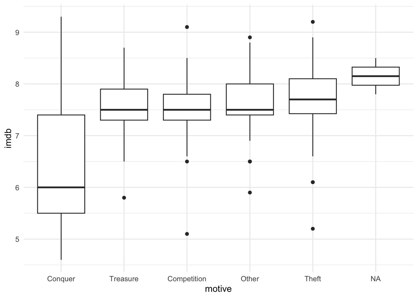
By default, fct_reorder sorts using the median. You can specify a different function (like mean) by adding a .fun argument.
Ordered factors
Occasionally you may encounter ordered factors, ones of class ord. For the most part, you can treat these like regular factors.
glimpse(diamonds)Rows: 53,940
Columns: 10
$ carat <dbl> 0.23, 0.21, 0.23, 0.29, 0.31, 0.24, 0.24, 0.26, 0.22, 0.23, 0.…
$ cut <ord> Ideal, Premium, Good, Premium, Good, Very Good, Very Good, Ver…
$ color <ord> E, E, E, I, J, J, I, H, E, H, J, J, F, J, E, E, I, J, J, J, I,…
$ clarity <ord> SI2, SI1, VS1, VS2, SI2, VVS2, VVS1, SI1, VS2, VS1, SI1, VS1, …
$ depth <dbl> 61.5, 59.8, 56.9, 62.4, 63.3, 62.8, 62.3, 61.9, 65.1, 59.4, 64…
$ table <dbl> 55, 61, 65, 58, 58, 57, 57, 55, 61, 61, 55, 56, 61, 54, 62, 58…
$ price <int> 326, 326, 327, 334, 335, 336, 336, 337, 337, 338, 339, 340, 34…
$ x <dbl> 3.95, 3.89, 4.05, 4.20, 4.34, 3.94, 3.95, 4.07, 3.87, 4.00, 4.…
$ y <dbl> 3.98, 3.84, 4.07, 4.23, 4.35, 3.96, 3.98, 4.11, 3.78, 4.05, 4.…
$ z <dbl> 2.43, 2.31, 2.31, 2.63, 2.75, 2.48, 2.47, 2.53, 2.49, 2.39, 2.…diamonds |>
count(cut) # several ordered factors# A tibble: 5 × 2
cut n
<ord> <int>
1 Fair 1610
2 Good 4906
3 Very Good 12082
4 Premium 13791
5 Ideal 21551Specifying that a factor is ordered (for instance using ordered) can occasionally matter in modeling applications and certain forms of statistical inference. Other than that, the most visible difference with ordered factors in R is how they’re displayed by ggplot.
ggplot(diamonds, aes(x = cut,
                     fill = cut)) +
  geom_bar(show.legend = FALSE)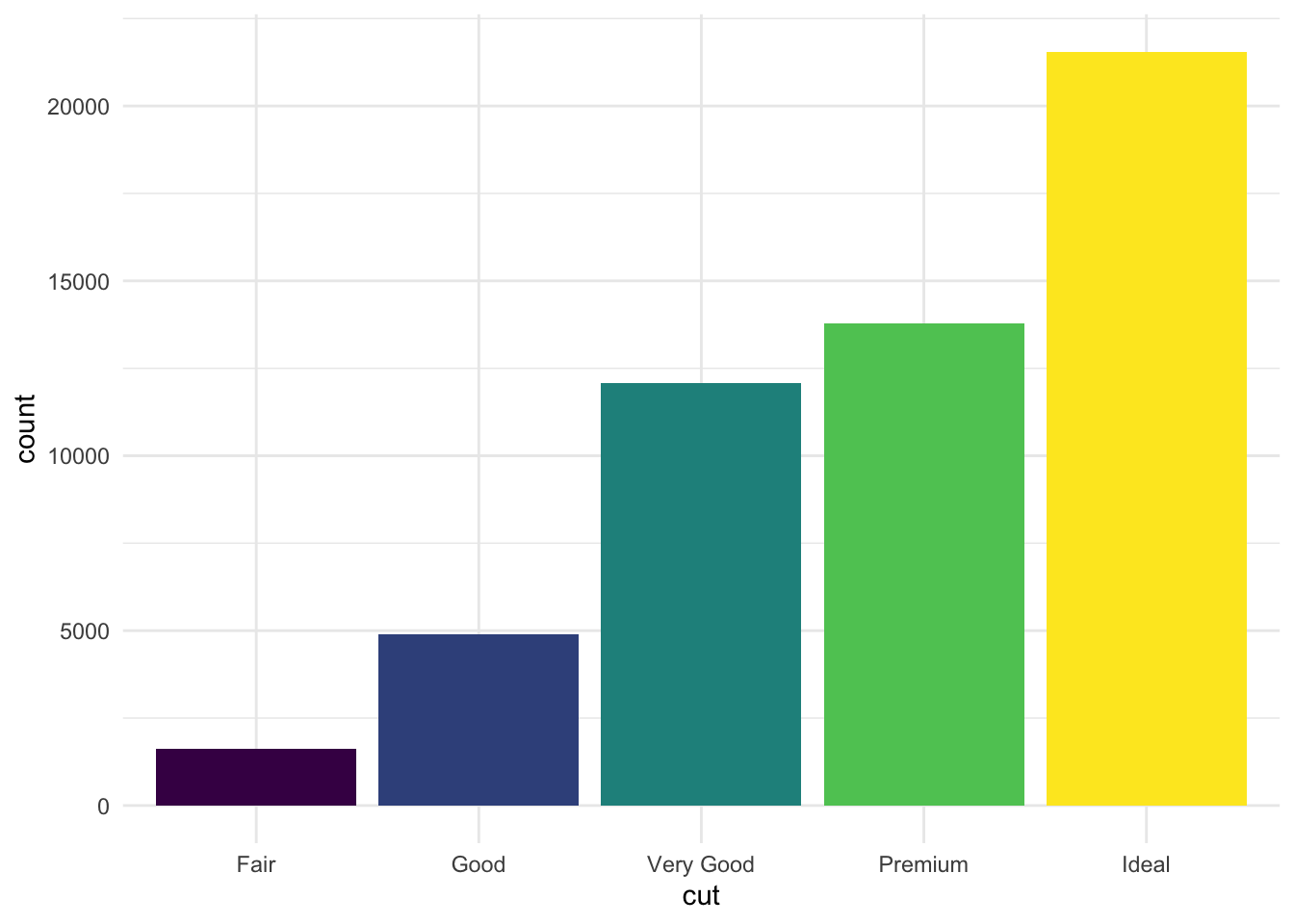
By default, ordered factors are colored using the viridis palette, which is has a distinct order to it.
Want more?
If something here isn’t clear, there’s a good chance you’ll find an explanation in my vid on the subject:
This post will be cross-listed on R-bloggers, a site that I totally recommend.