How to tidymodels

Pull up your socks! It’s time to tackle machine learning in R.

library(tidymodels)
library(ISLR2) 

The tidymodels family of packages is a unified framework for machine learning in R. I recommend it for predictive modeling, where future performance is the primary benchmark for success. For descriptive modeling and statistical inference, tidymodels can be unwieldy.

The College data set

Throughout this demonstration, I’ll use the ISLR2::College data set, which includes information about 777 US colleges in 1995 ¹. We’ll view Outstate tuition as the response variable, attempting to model it using the other variables in the set.

glimpse(College)

Rows: 777
Columns: 18
$ Private     <fct> Yes, Yes, Yes, Yes, Yes, Yes, Yes, Yes, Yes, Yes, Yes, Yes…
$ Apps        <dbl> 1660, 2186, 1428, 417, 193, 587, 353, 1899, 1038, 582, 173…
$ Accept      <dbl> 1232, 1924, 1097, 349, 146, 479, 340, 1720, 839, 498, 1425…
$ Enroll      <dbl> 721, 512, 336, 137, 55, 158, 103, 489, 227, 172, 472, 484,…
$ Top10perc   <dbl> 23, 16, 22, 60, 16, 38, 17, 37, 30, 21, 37, 44, 38, 44, 23…
$ Top25perc   <dbl> 52, 29, 50, 89, 44, 62, 45, 68, 63, 44, 75, 77, 64, 73, 46…
$ F.Undergrad <dbl> 2885, 2683, 1036, 510, 249, 678, 416, 1594, 973, 799, 1830…
$ P.Undergrad <dbl> 537, 1227, 99, 63, 869, 41, 230, 32, 306, 78, 110, 44, 638…
$ Outstate    <dbl> 7440, 12280, 11250, 12960, 7560, 13500, 13290, 13868, 1559…
$ Room.Board  <dbl> 3300, 6450, 3750, 5450, 4120, 3335, 5720, 4826, 4400, 3380…
$ Books       <dbl> 450, 750, 400, 450, 800, 500, 500, 450, 300, 660, 500, 400…
$ Personal    <dbl> 2200, 1500, 1165, 875, 1500, 675, 1500, 850, 500, 1800, 60…
$ PhD         <dbl> 70, 29, 53, 92, 76, 67, 90, 89, 79, 40, 82, 73, 60, 79, 36…
$ Terminal    <dbl> 78, 30, 66, 97, 72, 73, 93, 100, 84, 41, 88, 91, 84, 87, 6…
$ S.F.Ratio   <dbl> 18.1, 12.2, 12.9, 7.7, 11.9, 9.4, 11.5, 13.7, 11.3, 11.5, …
$ perc.alumni <dbl> 12, 16, 30, 37, 2, 11, 26, 37, 23, 15, 31, 41, 21, 32, 26,…
$ Expend      <dbl> 7041, 10527, 8735, 19016, 10922, 9727, 8861, 11487, 11644,…
$ Grad.Rate   <dbl> 60, 56, 54, 59, 15, 55, 63, 73, 80, 52, 73, 76, 74, 68, 55…

The models shown below were chosen for clarity of presentation, and there are many places where different choices could lead to better performance. If you’re serious about learning these tools, a helpful exercise would be to try beat the results shown at the end of this post.

A model with no holdout set or CV split

R comes with several built-in modeling functions, including lm(). Many more are included in add-on packages like glmnet, ranger, etc. They syntax of these packages is highly inconsistent.

The parsnip package, which loads with tidymodels, provides user-friendly wrapper functions for these tools, so in theory you don’t have to learn a new package every time you learn a new modeling technique. The inputs and outputs have consistent structure, facilitating preprocessing, tuning, and evaluation.

On the other hand, you can’t just plug a model formula into something like parsnip::linear_reg() and get coefficients back, as you would with lm().

linear_reg(Outstate ~ Top10perc, 
           data = College) # Nope.

Error in `linear_reg()`:
! unused argument (data = College)

Instead, you specify the form of the model (below, just linear regression for now), then fit it separately using data.

my_lm <- linear_reg()

lm_fit <- fit(
  my_lm,
  Outstate ~ Top10perc + PhD,
  data = College
  )

lm_fit

parsnip model object


Call:
stats::lm(formula = Outstate ~ Top10perc + PhD, data = data)

Coefficients:
(Intercept)    Top10perc          PhD  
    5202.71       114.05        28.83  

This is awkward and underwhelming because the model is so simple and the lm() syntax so familiar. Most modern models require more fine-grained control. For instance, we might apply coefficient shrinkage to address model instability (don’t worry if you don’t know what this means yet). The syntax doesn’t change much.

enet <- linear_reg(
  mixture = .5, 
  penalty = 1, 
  engine = "glmnet"
  )

enet

Linear Regression Model Specification (regression)

Main Arguments:
  penalty = 1
  mixture = 0.5

Computational engine: glmnet 

The engine argument identifies which function or package should be used to actually do the modeling. There are typically multiple options available. Here, I’ve specified an elastic net from the glmnet package.

By the way, when used directly, glmnet expects to be handed a separate model matrix and response vector. This workflow lets us ignore that potentially troublesome fact.

It’s possible to immediately fit a model like the one above, but the output is specific to the engine and may not be immediately useful.

enet_fit <- fit(
  enet,
  Outstate ~ Top10perc + PhD,
  data = College
  )

enet_fit 

parsnip model object


Call:  glmnet::glmnet(x = maybe_matrix(x), y = y, family = "gaussian",      alpha = ~0.5) 

   Df  %Dev Lambda
1   0  0.00 4522.0
2   1  3.61 4120.0
3   1  6.90 3754.0
4   1  9.88 3420.0
5   1 12.58 3117.0
6   1 15.00 2840.0
7   1 17.16 2587.0
8   1 19.07 2358.0
9   1 20.77 2148.0
10  2 22.34 1957.0
11  2 23.86 1783.0
12  2 25.17 1625.0
13  2 26.29 1481.0
14  2 27.25 1349.0
15  2 28.08 1229.0
16  2 28.78 1120.0
17  2 29.38 1021.0
18  2 29.88  929.9
19  2 30.31  847.3
20  2 30.68  772.0
21  2 30.99  703.4
22  2 31.25  640.9
23  2 31.47  584.0
24  2 31.65  532.1
25  2 31.81  484.8
26  2 31.94  441.8
27  2 32.05  402.5
28  2 32.14  366.8
29  2 32.21  334.2
30  2 32.28  304.5
31  2 32.33  277.4
32  2 32.38  252.8
33  2 32.42  230.3
34  2 32.45  209.9
35  2 32.47  191.2
36  2 32.49  174.2
37  2 32.51  158.8
38  2 32.53  144.7
39  2 32.54  131.8
40  2 32.55  120.1
41  2 32.56  109.4
42  2 32.57   99.7
43  2 32.57   90.8
44  2 32.58   82.8
45  2 32.58   75.4
46  2 32.59   68.7
47  2 32.59   62.6
48  2 32.59   57.1
49  2 32.59   52.0
50  2 32.60   47.4
51  2 32.60   43.2
52  2 32.60   39.3
53  2 32.60   35.8
54  2 32.60   32.6
55  2 32.60   29.8
56  2 32.60   27.1
57  2 32.60   24.7
58  2 32.60   22.5
59  2 32.60   20.5

The broom::tidy function is your friend if you want model coefficients and p-values.

tidy(lm_fit)

# A tibble: 3 × 5
  term        estimate std.error statistic  p.value
  <chr>          <dbl>     <dbl>     <dbl>    <dbl>
1 (Intercept)   5203.     553.        9.41 5.64e-20
2 Top10perc      114.       7.95     14.4  1.37e-41
3 PhD             28.8      8.59      3.36 8.23e- 4

tidy(enet_fit)

# A tibble: 3 × 3
  term        estimate penalty
  <chr>          <dbl>   <dbl>
1 (Intercept)   5243.        1
2 Top10perc      113.        1
3 PhD             28.6       1

You can make predictions using predict().

new_data = data.frame(
  Top10perc = c(20, 30, 40),
  PhD = c(70, 60, 80),
  Outstate = c(10000, 15000, 17000)
  )

predict(enet_fit, new_data)

# A tibble: 3 × 1
   .pred
   <dbl>
1  9508.
2 10356.
3 12060.

While nice, none of this is really worth the overhead of learning tidymodels. The primary advantage of the above workflow is the ease with which we can add data splitting, preprocessing, parameter tuning, and model evaluation.

Machine learning with tidymodels

The tidymodels framework starts to shine when we use it for machine learning, where future performance of the model is prioritized over interpretability or statistical inference.

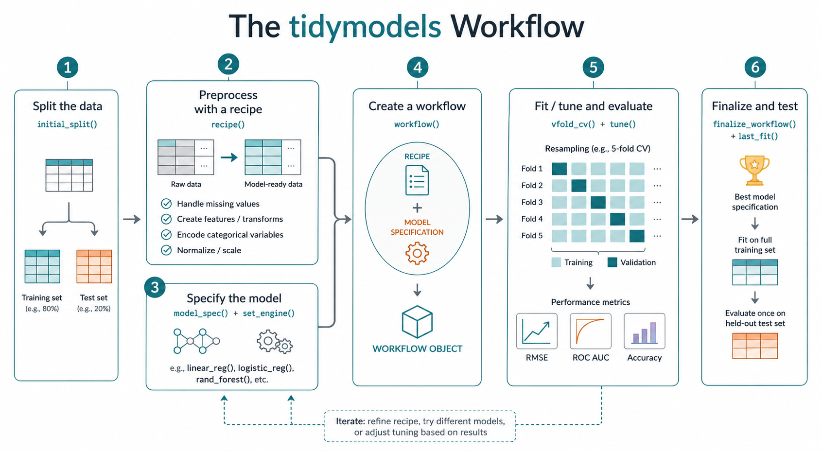
When using data to estimate the future performance of a model, we always adhere to one essential core principle, which tidymodels works hard to enforce:

\[ \text{\textbf{Do not use the same data to both train and assess any model.}} \]

At the start of the modeling process, then, we set aside a fraction of our observations (usually 20% or 25%) for final evaluation, using the remaining ones for model building. Additional splits are often needed when the model is being tuned. More on this later.

Splitting the data

The rsample::initial_split() function partitions a data set by randomly assigning rows (prop = 3/4 is the default) to the training set and storing them, along with the full data frame, in a list (technically, an rsplit object).

set.seed(0)

split <- initial_split(College)
split

<Training/Testing/Total>
<582/195/777>

names(split)

[1] "data"   "in_id"  "out_id" "id"    

split$in_id |> head(n = 20)

 [1] 398 679 129 509 471 299 270 187 307 597 277 494 330 591 725  37 105 729 485
[20] 677

The training set, then, is split$data[split$in_id, ], though tidymodels provides simple functions to extract both the training and testing sets.

train <- training(split)
test <- testing(split)

glimpse(train) # 582 rows, ~75% of the original set

Rows: 582
Columns: 18
$ Private     <fct> Yes, No, Yes, No, Yes, Yes, No, Yes, Yes, Yes, Yes, Yes, Y…
$ Apps        <dbl> 657, 1401, 344, 4216, 427, 2929, 8681, 1457, 1243, 2425, 4…
$ Accept      <dbl> 537, 1239, 264, 2290, 385, 1834, 6695, 1045, 947, 1818, 35…
$ Enroll      <dbl> 113, 605, 97, 736, 143, 622, 2408, 345, 324, 601, 913, 225…
$ Top10perc   <dbl> 37, 10, 11, 20, 18, 20, 10, 27, 50, 62, 13, 24, 25, 57, 42…
$ Top25perc   <dbl> 90, 34, 42, 52, 38, 56, 35, 50, 77, 93, 33, 42, 55, 81, 64…
$ F.Undergrad <dbl> 1039, 3716, 500, 4296, 581, 2738, 15701, 1109, 1129, 2110,…
$ P.Undergrad <dbl> 466, 675, 331, 1027, 533, 1662, 1823, 502, 74, 95, 1446, 2…
$ Outstate    <dbl> 12474, 7100, 12600, 5130, 12700, 12600, 7799, 14990, 17163…
$ Room.Board  <dbl> 5678, 4380, 5520, 4690, 5800, 5610, 3403, 4980, 3891, 5150…
$ Books       <dbl> 630, 540, 630, 600, 450, 450, 537, 450, 525, 500, 570, 600…
$ Personal    <dbl> 1278, 2948, 2250, 1450, 700, 3160, 2605, 550, 975, 490, 11…
$ PhD         <dbl> 53, 63, 77, 73, 81, 90, 77, 77, 76, 94, 66, 55, 94, 81, 91…
$ Terminal    <dbl> 71, 88, 80, 75, 85, 90, 84, 98, 92, 96, 83, 60, 95, 91, 91…
$ S.F.Ratio   <dbl> 11.9, 19.4, 10.4, 17.9, 10.3, 15.1, 21.0, 21.5, 10.1, 9.6,…
$ perc.alumni <dbl> 19, 0, 7, 18, 37, 9, 16, 21, 57, 20, 14, 19, 15, 41, 40, 3…
$ Expend      <dbl> 10613, 5389, 9773, 5125, 11758, 9084, 5569, 7502, 13965, 1…
$ Grad.Rate   <dbl> 72, 36, 43, 56, 84, 84, 54, 64, 77, 93, 66, 67, 65, 70, 86…

We could also consider stratifying the split by the response variable. If the response is quantitative, as is the case here, initial_split() will automatically group it into quartiles.

split <- initial_split(
  College, 
  strata = Outstate
  )

One advantage to retaining the rsplit object rather than just creating train and test directly (for instance with slice_sample and anti_join) is that tidymodels will later allow us to effortlessly apply model assessment functions to the split object itself.

For now we leave the test set aside and build the model entirely using train.

Specifying the model

It’s time to decide how we’ll model the data. Let’s start with a simple \(k\)-nearest neighbor regression, where the closest points to a new observation are used to estimate an unknown response value. For this, we use parsnip::nearest_neighbor().

To start, we can just pick a reasonable value for the number of neighbors, \(k\). Sometimes \(k = \sqrt{n}\) is recommended, so we pick a value close to that. Later, we should consider whether other values might give better results.

my_knn <- nearest_neighbor(
  mode = "regression",
  engine = "kknn",
  neighbors = 27
  )

In this case, kknn::kknn() is the default engine; I’ve included the argument for clarity.

The mode of the model is typically either “regression” for a quantitative response or “classification” for a nominal one. In general, tidymodels will guess appropriately, so this argument is usually optional as well.

Preprocessing

Because this model will judge “nearest” using Pythagorean distance, it will be sensitive to the scale of the variables in the data set. Values measured in cents will appear 100 times farther apart than values measured in dollars, for instance.

For this reason, it’s considered best-practice to standardize all variables before fitting a knn model. This is a simple form of preprocessing, transforming existing variables to obtain something more amenable to the chosen modeling technique. While such work can be done directly with dplyr, there is a better way.

A recipe, as the name suggests, is a documented set of steps to be followed when any data (training, test, or otherwise) is handled by a model. Storing our steps in this way allows us to automate the process so that it be easily applied as needed.

Let’s create a simple recipe appropriate to a knn model.

col_rec <- recipe(Outstate ~ ., data = train) |> 
  step_dummy(all_nominal_predictors()) |> 
  step_normalize(all_numeric_predictors())

Preprocessing tools generally have the form step_*(). Most common techniques have built-in functions, including the two used above.

• step_dummy() encodes the specified categorical variables (here, all categorical explainers) as dummy variables. While some modeling functions (including our old friend lm) do this automatically, tidymodels requires that we be explicit.

• step_normalize() converts values to \(z\)-scores using the sample mean and standard deviation from the training set, placing them onto a common scale.

These are two common and important preprocessing tools. There are many more, including ones that perform feature engineering, extracting important information that may not be captured directly by existing variables. For instance, in a set that includes dates, the day of the week may the most relevant aspect. This can be extracted with step_date().

Just as tidymodels requires us to explicitly encode factor variables for numerical models, so does it require us to engage with missing values. This extra step is a very good thing, as it prevents us from casually dropping incomplete observations wholesale. NAs can be converted to an “unknown” category with step_unknown() or replaced with reasonable values using one of the various step_impute_*() functions.

In a moment, we’ll integrate our recipe directly into our modeling workflow. First, though, let’s consider what we already have.

You may have noticed that some steps (including step_normalize) require input from the training set. Currently the recipe, which is just a set of instructions, has not performed any such computations. Use prep() to tell tidymodels to incorporate the training data into the recipe.

rec_prepped <- prep(col_rec)
rec_prepped

── Recipe ──────────────────────────────────────────────────────────────────────

── Inputs 

Number of variables by role

outcome:    1
predictor: 17

── Training information 

Training data contained 582 data points and no incomplete rows.

── Operations 

• Dummy variables from: Private | Trained

• Centering and scaling for: Apps, Accept, Enroll, Top10perc, ... | Trained

The word “Trained” in the output refers to the recipe, not the overall model. For instance, our output indicates that \(z\)-scores have been computed using \(\overline{x}\) and \(s\) from the training set, where previously only the instruction to do so had existed.

Once the recipe is trained (prepped), it can be applied to any set with the correct column names, including train and test. For instance, the next chunk outputs a data frame showing the results of applying the recipe directly to the training set

train_baked <- bake(
  rec_prepped,
  new_data = train
  )

glimpse(train_baked)

Rows: 582
Columns: 18
$ Apps        <dbl> -0.584565901, -0.392108788, -0.665532402, 0.336072357, -0.…
$ Accept      <dbl> -0.59303713, -0.29578081, -0.70863680, 0.14925677, -0.6574…
$ Enroll      <dbl> -0.73007850, -0.16151757, -0.74856828, -0.01013245, -0.695…
$ Top10perc   <dbl> 0.53780784, -1.01427892, -0.95679422, -0.43943197, -0.5544…
$ Top25perc   <dbl> 1.718305395, -1.097897433, -0.695582743, -0.192689381, -0.…
$ F.Undergrad <dbl> -0.54793004, 0.03889871, -0.66608495, 0.16604129, -0.64832…
$ P.Undergrad <dbl> -0.25540460, -0.12116108, -0.34211693, 0.10493328, -0.2123…
$ Room.Board  <dbl> 1.1778784439, -0.0004757491, 1.0344424173, 0.2809493663, 1…
$ Books       <dbl> 0.45651909, -0.07400850, 0.45651909, 0.27967656, -0.604536…
$ Personal    <dbl> -0.08996942, 2.29903910, 1.30051937, 0.15608415, -0.916823…
$ PhD         <dbl> -1.21449875, -0.59630890, 0.26915688, 0.02188095, 0.516432…
$ Terminal    <dbl> -0.60448281, 0.56500349, 0.01465699, -0.32930956, 0.358623…
$ S.F.Ratio   <dbl> -0.54144438, 1.38707844, -0.92714895, 1.00137388, -0.95286…
$ perc.alumni <dbl> -0.30283014, -1.84957177, -1.27971959, -0.38423759, 1.1625…
$ Expend      <dbl> 0.164258830, -0.812840693, 0.007144818, -0.862219382, 0.37…
$ Grad.Rate   <dbl> 0.39369765, -1.70682518, -1.29839018, -0.53986805, 1.09387…
$ Outstate    <dbl> 12474, 7100, 12600, 5130, 12700, 12600, 7799, 14990, 17163…
$ Private_Yes <dbl> 0.5913933, -1.6880167, 0.5913933, -1.6880167, 0.5913933, 0…

If we were to bake a recipe using some other new_data, \(z\)-scores would still be computed using means and standard deviations from the training set.

In general, you only need prep() and bake() if you want to explicitly see the transformed predictors. More typically, we just incorporate the preprocessor directly into a tidymodels workflow.

Creating a workflow

A workflow incorporates both a recipe and a model specification.

knn_wf <- workflow(
  preprocessor = col_rec,
  spec = my_knn
  )

Often, you’ll see this step written using the pipe.

knn_wf <- workflow() |> 
  add_recipe(col_rec) |> 
  add_model(my_knn) # same as before

It’s common in tidymodels to pipe various model objects, connecting them like pieces of a ggplot call. For instance, a model is often specified like this:

my_knn <- nearest_neighbor() |> 
  set_engine("kknn") |> 
  set_mode("regression") # same as before

This may feel awkward if you’re used to only piping data sets. You get past that quickly, I promise.

A workflow is a combined set of instructions for fitting a model to data. It says how to preprocess that data and constructs an algorithm for making predictions on new observations. Importantly, it does not actually execute any of those steps, still putting off the fitting process.

knn_wf

══ Workflow ════════════════════════════════════════════════════════════════════
Preprocessor: Recipe
Model: nearest_neighbor()

── Preprocessor ────────────────────────────────────────────────────────────────
2 Recipe Steps

• step_dummy()
• step_normalize()

── Model ───────────────────────────────────────────────────────────────────────
K-Nearest Neighbor Model Specification (regression)

Main Arguments:
  neighbors = 27

Computational engine: kknn 

We can take this next step using the fit() function, which we’ve seen before.

knn_wf_fit <- fit(
  knn_wf, 
  data = train
  )

The model is now ready to use.

Putting a trained workflow into action

Use predict() to make predictions, duh. To start, we might just look at the training set, checking how far actual results are from the model’s predictions. The output is a tibble, not a vector.

predict(
  knn_wf_fit, 
  new_data = train
  )

# A tibble: 582 × 1
    .pred
    <dbl>
 1 10953.
 2  6386.
 3 11191.
 4  6389.
 5 12944.
 6 12481.
 7  7213.
 8 12128.
 9 15024.
10 16666.
# ℹ 572 more rows

Predictions made on the same data used to train the model will almost always be overly optimistic. It’s like when your mom tells you that you look nice.

Evaluation using the test set

Once we’ve finalized our model, we can check its performance on the holdout set.

Warning! Using the results of this check to tweak the model would invalidate the point of the testing set, which is to give a measure of performance independent from the training data. In general, you shouldn’t do it.

The broom::augment() function makes this information readily available in a data frame that includes all the variables relevant to the model.

test_aug <- augment(
  knn_wf_fit, 
  new_data = test
  )

glimpse(test_aug)

Rows: 195
Columns: 20
$ .pred       <dbl> 13336.612, 8703.528, 14329.337, 11667.361, 13250.051, 9757…
$ .resid      <dbl> 2258.3878, 1764.4716, 2750.6630, -1977.3613, -678.0513, 14…
$ Private     <fct> Yes, Yes, Yes, Yes, Yes, Yes, No, No, Yes, Yes, No, Yes, Y…
$ Apps        <dbl> 1038, 582, 2652, 1179, 1267, 619, 12809, 1734, 1879, 2496,…
$ Accept      <dbl> 839, 498, 1900, 780, 1080, 516, 10308, 1729, 1658, 1402, 8…
$ Enroll      <dbl> 227, 172, 484, 290, 385, 219, 3761, 951, 497, 531, 546, 48…
$ Top10perc   <dbl> 30, 21, 44, 38, 44, 20, 24, 12, 36, 53, 12, 37, 11, 15, 20…
$ Top25perc   <dbl> 63, 44, 77, 64, 73, 51, 49, 52, 69, 95, 36, 68, 28, 55, 50…
$ F.Undergrad <dbl> 973, 799, 1707, 1130, 1306, 1251, 22593, 3602, 1950, 2121,…
$ P.Undergrad <dbl> 306, 78, 44, 638, 28, 767, 7585, 939, 38, 69, 824, 49, 74,…
$ Outstate    <dbl> 15595, 10468, 17080, 9690, 12572, 11208, 7434, 3460, 13353…
$ Room.Board  <dbl> 4400, 3380, 4440, 4785, 4552, 4124, 4850, 2650, 4173, 8124…
$ Books       <dbl> 300, 660, 400, 600, 400, 350, 700, 450, 540, 600, 660, 350…
$ Personal    <dbl> 500, 1800, 600, 1000, 400, 1615, 2100, 1000, 821, 850, 180…
$ PhD         <dbl> 79, 40, 73, 60, 79, 55, 88, 57, 78, 83, 57, 80, 63, 66, 76…
$ Terminal    <dbl> 84, 41, 91, 84, 87, 65, 93, 60, 83, 93, 62, 80, 63, 68, 71…
$ S.F.Ratio   <dbl> 11.3, 11.5, 9.9, 13.3, 15.3, 12.7, 18.9, 19.6, 12.7, 10.3,…
$ perc.alumni <dbl> 23, 15, 41, 21, 32, 25, 5, 5, 40, 33, 16, 17, 13, 19, 19, …
$ Expend      <dbl> 11644, 8991, 11711, 7940, 9305, 6584, 4602, 4739, 9220, 12…
$ Grad.Rate   <dbl> 80, 52, 76, 74, 68, 65, 48, 48, 71, 91, 46, 63, 35, 75, 58…

The yardstick package, included in tidymodels, consists of dedicated functions for computing standard performance metrics, including root mean squared error and \(R^2\). There are dozens of such functions available, all with consistent syntax. See the package index file for a complete list.

rmse(test_aug, 
     truth = Outstate,
     estimate = .pred)

# A tibble: 1 × 3
  .metric .estimator .estimate
  <chr>   <chr>          <dbl>
1 rmse    standard       1905.

You can compute multiple performance metrics at once by creating a metric set.

my_metrics <- metric_set(rmse, rsq)

my_metrics(
  test_aug,
  truth = Outstate, 
  estimate = .pred
  )

# A tibble: 2 × 3
  .metric .estimator .estimate
  <chr>   <chr>          <dbl>
1 rmse    standard    1905.   
2 rsq     standard       0.767

The fact that these outputs are tibbles will be very convenient once we begin comparing various models.

Model tuning and cross validation

It’s unlikely that our choice of \(k=27\) neighbors was optimal. Model tuning refers to the process of considering a range of hyperparameter values and selecting the best one. tidymodels is built to facilitate it.

We start by specifying within our model that a hyperparameter needs to be tuned. We do this with the tune() placeholder.

my_knn_cv <- nearest_neighbor(
  mode = "regression",
  engine = "kknn",
  neighbors = tune()
  )

knn_wf_cv <- workflow(
  preprocessor = col_rec,
  spec = my_knn_cv
  )

The most common way of comparing competing models during the tuning process is using cross-validation, where the training set is split into pieces (often \(v=10\)) of approximately equal size, called folds. The models are all then trained once per fold, with that one fold used as a holdout set while the others are used for training. The \(v\) results (measured using rmse or some other metric) are then averaged to give performance estimates for each of the competing models.

We create the cross validation split using rsample::vfold_cv(). The output is a tibble with one row per fold.

folds <- vfold_cv(
  train, 
  v = 10,
  repeats = 5)

head(folds)

# A tibble: 6 × 3
  splits           id      id2   
  <list>           <chr>   <chr> 
1 <split [523/59]> Repeat1 Fold01
2 <split [523/59]> Repeat1 Fold02
3 <split [524/58]> Repeat1 Fold03
4 <split [524/58]> Repeat1 Fold04
5 <split [524/58]> Repeat1 Fold05
6 <split [524/58]> Repeat1 Fold06

The repeats argument indicates that the 10-fold split should be done 5 separate times, meaning that we’re about to fit our model 50 times as part of our tuning process. This may become time-consuming, even on a modern computer. While repeats aren’t strictly required, using them reduces the variance (uncertainty) of the cross-validation result.

The simplest tool to perform model fitting on cross-validation folds is tune_grid().

tune_results <- tune_grid(
  knn_wf_cv,
  resamples = folds
  )

This function operates by brute force using a default set of 10 values that make sense for the hyperparameter being tuned. Often, you’ll want to tweak these values using the optional grid argument. You can either pass this as a data frame of parameter values or a dials object such as the one created by the neighbors() function. For this simple example, let’s use the first method.

neighbors <- seq(11, 33, by = 2)
knn_grid <- data.frame(neighbors)
knn_grid

   neighbors
1         11
2         13
3         15
4         17
5         19
6         21
7         23
8         25
9         27
10        29
11        31
12        33

tune_results <- tune_grid(
  knn_wf_cv,
  resamples = folds,
  grid = knn_grid
  )

glimpse(tune_results)

Rows: 50
Columns: 5
$ splits   <list> [<vfold_split[523 x 59 x 582 x 18]>], [<vfold_split[523 x 59…
$ id       <chr> "Repeat1", "Repeat1", "Repeat1", "Repeat1", "Repeat1", "Repea…
$ id2      <chr> "Fold01", "Fold02", "Fold03", "Fold04", "Fold05", "Fold06", "…
$ .metrics <list> [<tbl_df[24 x 5]>], [<tbl_df[24 x 5]>], [<tbl_df[24 x 5]>], …
$ .notes   <list> [<tbl_df[0 x 4]>], [<tbl_df[0 x 4]>], [<tbl_df[0 x 4]>], [<t…

The result is a mutated version of the output of vfold_cv() that includes new columns for .metrics and .notes. The first of these includes rmse and \(R^2\) for each parameter value on each fold. If you’d like to specify different measures of fit, create a metric set and use the optional metrics argument in tune_grid().

While it’s possible to drill down into the tune_results() object directly (it’s just a tibble, after all), you’ll usually want to either compare the overall performance of various hyperparameter values or just grab the best one directly. Use collect_metrics() to accomplish the former.

tuning_metrics <- collect_metrics(tune_results)
tuning_metrics

# A tibble: 24 × 7
   neighbors .metric .estimator     mean     n  std_err .config         
       <dbl> <chr>   <chr>         <dbl> <int>    <dbl> <chr>           
 1        11 rmse    standard   1944.       50 30.6     pre0_mod01_post0
 2        11 rsq     standard      0.770    50  0.00895 pre0_mod01_post0
 3        13 rmse    standard   1927.       50 30.6     pre0_mod02_post0
 4        13 rsq     standard      0.774    50  0.00900 pre0_mod02_post0
 5        15 rmse    standard   1917.       50 30.7     pre0_mod03_post0
 6        15 rsq     standard      0.777    50  0.00905 pre0_mod03_post0
 7        17 rmse    standard   1910.       50 30.8     pre0_mod04_post0
 8        17 rsq     standard      0.778    50  0.00911 pre0_mod04_post0
 9        19 rmse    standard   1906.       50 30.8     pre0_mod05_post0
10        19 rsq     standard      0.780    50  0.00914 pre0_mod05_post0
# ℹ 14 more rows

It’s often helpful to plot tuning results:

tuning_metrics |> 
  filter(.metric == "rmse") |> 
  ggplot(aes(x = neighbors, y = mean)) + 
  geom_line() +
  geom_point() +
  theme_minimal()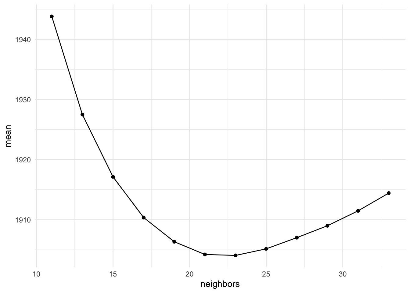

Use show_best() to automatically filter out sub-optimal rows from tuning_metrics. By default, the best 5 are shown, though this can be controlled with the optional n argument.

show_best(
  tune_results,
  metric = "rmse",
  n = 7
  ) 

# A tibble: 7 × 7
  neighbors .metric .estimator  mean     n std_err .config         
      <dbl> <chr>   <chr>      <dbl> <int>   <dbl> <chr>           
1        23 rmse    standard   1904.    50    30.7 pre0_mod07_post0
2        21 rmse    standard   1904.    50    30.7 pre0_mod06_post0
3        25 rmse    standard   1905.    50    30.6 pre0_mod08_post0
4        19 rmse    standard   1906.    50    30.8 pre0_mod05_post0
5        27 rmse    standard   1907.    50    30.5 pre0_mod09_post0
6        29 rmse    standard   1909.    50    30.5 pre0_mod10_post0
7        17 rmse    standard   1910.    50    30.8 pre0_mod04_post0

To automatically extract the result that minimizes rmse (or any other metric), use select_best().

optimal_k <- select_best(
  tune_results,
  metric = "rmse"
  )

optimal_k # 23 neighbors

# A tibble: 1 × 2
  neighbors .config         
      <dbl> <chr>           
1        23 pre0_mod07_post0

select_best() has several friends, including select_by_one_std_error(), which chooses the least flexible model with performance comparable to the optimal one.

The output of select_best() can be fed back to the workflow being tuned with finalize_workflow().

knn_wf_final <- finalize_workflow(
  knn_wf_cv,
  optimal_k
  )

knn_wf_final

══ Workflow ════════════════════════════════════════════════════════════════════
Preprocessor: Recipe
Model: nearest_neighbor()

── Preprocessor ────────────────────────────────────────────────────────────────
2 Recipe Steps

• step_dummy()
• step_normalize()

── Model ───────────────────────────────────────────────────────────────────────
K-Nearest Neighbor Model Specification (regression)

Main Arguments:
  neighbors = 23

Computational engine: kknn 

The model is now fully specified.

Evaluating performance

We can incorporate training data into our finalized model with fit(). The output can be saved and applied to new data with predict().

knn_final <- fit(
  knn_wf_final, 
  data = train
  )

predict(
  knn_final, 
  new_data = test
  )

# A tibble: 195 × 1
    .pred
    <dbl>
 1 13404.
 2  8653.
 3 14218.
 4 11709.
 5 13200.
 6  9714.
 7  7556.
 8  4981.
 9 13158.
10 18405.
# ℹ 185 more rows

If all you want to do is apply the trained model to the holdout set created with initial_split(), use last_fit(). To extract performance metrics from this object, use collect_metrics().

last_fit(knn_wf_final, split) |>
  collect_metrics()

# A tibble: 2 × 4
  .metric .estimator .estimate .config        
  <chr>   <chr>          <dbl> <chr>          
1 rmse    standard    1904.    pre0_mod0_post0
2 rsq     standard       0.767 pre0_mod0_post0

On average, this model misses the true out-of-state tuition by about $1904.

What’s next?

This post barely scratches the surface, despite its length. If you’ve made it this far, you might be itching to compare the performance of other models (like neural networks, for instance) or alternative preprocessing steps. This can be done with a workflow_set. Or you might want to speed up the tuning process, either by using a less brute-force approach from the tune package, most notably tune_Bayes(), or by implementing parallel processing for the calculations using the future package.

Final thought

If you were expecting that learning tidymodels would be like learning tidyverse, you’re probably disappointed right about now. While you can practice dplyr without touching ggplot2, you can’t meaningfully do this with the individual tidymodels packages. This isn’t a design flaw in tidymodels but rather a fundamental challenge of the machine learning process, which is interconnected and complex by its very nature.

Overall, tidymodels is as about as simple as it can be while still doing what it does. Be patient with yourself, take multiple passes at the content, and you’ll get there sooner than you think.

Footnotes

1. James, G., Witten, D., Hastie, T., & Tibshirani, R. (2021). An introduction to statistical learning: with applications in R (Vol. 2). https://www.statlearning.com/