library(tidymodels)
library(ISLR2)
# glmnet must also be installed but need not be loaded

set.seed(0) # For reproducibility
Ridge regression in R
Machine learning
tidymodels
Today I’m modeling college graduation rates using ridge regression. I’m not a nerd, you’re the nerd.
Ridge regression addresses model instability by pushing coefficients slightly toward zero. Check out this video for a deeper explanation of why this might be desirable. TL/DR: it’s the bias-variance tradeoff.
In this post, I’ll model graduation rates at various US colleges using the ISLR2::College data set. We start by splitting the data.
split <- initial_split(College)
split # 582 training obs, 195 testing obs
<Training/Testing/Total>
<582/195/777>train <- training(split)
test <- testing(split)
glimpse(train)Rows: 582
Columns: 18
$ Private <fct> Yes, No, Yes, No, Yes, Yes, No, Yes, Yes, Yes, Yes, Yes, Y…
$ Apps <dbl> 657, 1401, 344, 4216, 427, 2929, 8681, 1457, 1243, 2425, 4…
$ Accept <dbl> 537, 1239, 264, 2290, 385, 1834, 6695, 1045, 947, 1818, 35…
$ Enroll <dbl> 113, 605, 97, 736, 143, 622, 2408, 345, 324, 601, 913, 225…
$ Top10perc <dbl> 37, 10, 11, 20, 18, 20, 10, 27, 50, 62, 13, 24, 25, 57, 42…
$ Top25perc <dbl> 90, 34, 42, 52, 38, 56, 35, 50, 77, 93, 33, 42, 55, 81, 64…
$ F.Undergrad <dbl> 1039, 3716, 500, 4296, 581, 2738, 15701, 1109, 1129, 2110,…
$ P.Undergrad <dbl> 466, 675, 331, 1027, 533, 1662, 1823, 502, 74, 95, 1446, 2…
$ Outstate <dbl> 12474, 7100, 12600, 5130, 12700, 12600, 7799, 14990, 17163…
$ Room.Board <dbl> 5678, 4380, 5520, 4690, 5800, 5610, 3403, 4980, 3891, 5150…
$ Books <dbl> 630, 540, 630, 600, 450, 450, 537, 450, 525, 500, 570, 600…
$ Personal <dbl> 1278, 2948, 2250, 1450, 700, 3160, 2605, 550, 975, 490, 11…
$ PhD <dbl> 53, 63, 77, 73, 81, 90, 77, 77, 76, 94, 66, 55, 94, 81, 91…
$ Terminal <dbl> 71, 88, 80, 75, 85, 90, 84, 98, 92, 96, 83, 60, 95, 91, 91…
$ S.F.Ratio <dbl> 11.9, 19.4, 10.4, 17.9, 10.3, 15.1, 21.0, 21.5, 10.1, 9.6,…
$ perc.alumni <dbl> 19, 0, 7, 18, 37, 9, 16, 21, 57, 20, 14, 19, 15, 41, 40, 3…
$ Expend <dbl> 10613, 5389, 9773, 5125, 11758, 9084, 5569, 7502, 13965, 1…
$ Grad.Rate <dbl> 72, 36, 43, 56, 84, 84, 54, 64, 77, 93, 66, 67, 65, 70, 86…Since we’ll be using tidymodels, we need to create a model specification (basically a custom modeling function) and a recipe (instructions for preprocessing) before bundling the two together into a workflow.
my_ridge <- linear_reg(
  engine = "glmnet",
  mixture = 0, # zero for ridge, one for lasso
  penalty = tune())

my_rec <- recipe(Grad.Rate ~., data = train) |>
  step_zv(all_predictors()) |>
  step_dummy(all_nominal_predictors()) |>
  step_normalize(all_numeric_predictors())

my_wf <- workflow(spec = my_ridge,
                  preprocessor = my_rec)
When we fit our model, our preprocessing steps will be automatically applied. When we make predictions, the workflow will know when to use training data (for instance in computing means and sds for z-scores) and when to use new observations. Tidymodels is built to prevent data leakage, which is one if its main features.
Next we identify a good penalty value using cross validation.
# create split
folds <- vfold_cv(
  train,
  v = 10,
  repeats = 5)
folds # 10 folds 5 times for 50 rows
# 10-fold cross-validation repeated 5 times
# A tibble: 50 × 3
splits id id2
<list> <chr> <chr>
1 <split [523/59]> Repeat1 Fold01
2 <split [523/59]> Repeat1 Fold02
3 <split [524/58]> Repeat1 Fold03
4 <split [524/58]> Repeat1 Fold04
5 <split [524/58]> Repeat1 Fold05
6 <split [524/58]> Repeat1 Fold06
7 <split [524/58]> Repeat1 Fold07
8 <split [524/58]> Repeat1 Fold08
9 <split [524/58]> Repeat1 Fold09
10 <split [524/58]> Repeat1 Fold10
# ℹ 40 more rowstune_results <- tune_grid(
my_wf,
folds
)
tune_results # 10 results per fold per rep# Tuning results
# 10-fold cross-validation repeated 5 times
# A tibble: 50 × 5
splits id id2 .metrics .notes
<list> <chr> <chr> <list> <list>
1 <split [523/59]> Repeat1 Fold01 <tibble [20 × 5]> <tibble [0 × 4]>
2 <split [523/59]> Repeat1 Fold02 <tibble [20 × 5]> <tibble [0 × 4]>
3 <split [524/58]> Repeat1 Fold03 <tibble [20 × 5]> <tibble [0 × 4]>
4 <split [524/58]> Repeat1 Fold04 <tibble [20 × 5]> <tibble [0 × 4]>
5 <split [524/58]> Repeat1 Fold05 <tibble [20 × 5]> <tibble [0 × 4]>
6 <split [524/58]> Repeat1 Fold06 <tibble [20 × 5]> <tibble [0 × 4]>
7 <split [524/58]> Repeat1 Fold07 <tibble [20 × 5]> <tibble [0 × 4]>
8 <split [524/58]> Repeat1 Fold08 <tibble [20 × 5]> <tibble [0 × 4]>
9 <split [524/58]> Repeat1 Fold09 <tibble [20 × 5]> <tibble [0 × 4]>
10 <split [524/58]> Repeat1 Fold10 <tibble [20 × 5]> <tibble [0 × 4]>
# ℹ 40 more rowstune_results$.metrics[[1]] # results for fold 1 rep 1# A tibble: 20 × 5
penalty .metric .estimator .estimate .config
<dbl> <chr> <chr> <dbl> <chr>
1 1.02e-10 rmse standard 11.4 pre0_mod01_post0
2 1.02e-10 rsq standard 0.442 pre0_mod01_post0
3 1.28e- 9 rmse standard 11.4 pre0_mod02_post0
4 1.28e- 9 rsq standard 0.442 pre0_mod02_post0
5 7.19e- 9 rmse standard 11.4 pre0_mod03_post0
6 7.19e- 9 rsq standard 0.442 pre0_mod03_post0
7 4.55e- 8 rmse standard 11.4 pre0_mod04_post0
8 4.55e- 8 rsq standard 0.442 pre0_mod04_post0
9 3.69e- 7 rmse standard 11.4 pre0_mod05_post0
10 3.69e- 7 rsq standard 0.442 pre0_mod05_post0
11 3.14e- 6 rmse standard 11.4 pre0_mod06_post0
12 3.14e- 6 rsq standard 0.442 pre0_mod06_post0
13 7.73e- 5 rmse standard 11.4 pre0_mod07_post0
14 7.73e- 5 rsq standard 0.442 pre0_mod07_post0
15 1.30e- 3 rmse standard 11.4 pre0_mod08_post0
16 1.30e- 3 rsq standard 0.442 pre0_mod08_post0
17 2.44e- 2 rmse standard 11.4 pre0_mod09_post0
18 2.44e- 2 rsq standard 0.442 pre0_mod09_post0
19 7.71e- 1 rmse standard 11.4 pre0_mod10_post0
20 7.71e- 1 rsq standard 0.442 pre0_mod10_post0rmse_path <- collect_metrics(tune_results) |>
filter(.metric == "rmse")
ggplot(rmse_path, aes(x = penalty,
y = mean)) +
geom_point() +
geom_line()+
scale_x_log10(labels = scales::label_log()) +
labs(x = "Penalty (log scale)",
y = "CV error") +
theme_minimal()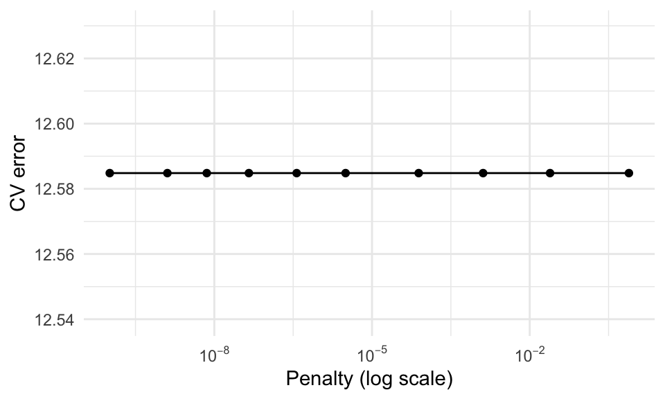
The default range for \(lambda\) doesn’t appear to include the ideal value. We need to consider larger values until we see RMSE begin to increase.
my_grid <- data.frame(
  penalty = 10^seq(-1, 1, length.out = 20)
)

tune_results <- tune_grid(
  my_wf,
  folds,
  grid = my_grid
)

rmse_path <- collect_metrics(tune_results) |>
  filter(.metric == "rmse")

ggplot(rmse_path, aes(x = penalty,
                      y = mean)) +
  geom_point() +
  geom_line()+
  scale_x_log10(labels = scales::label_log()) +
  labs(x = "Penalty",
       y = "Test error") +
  theme_minimal()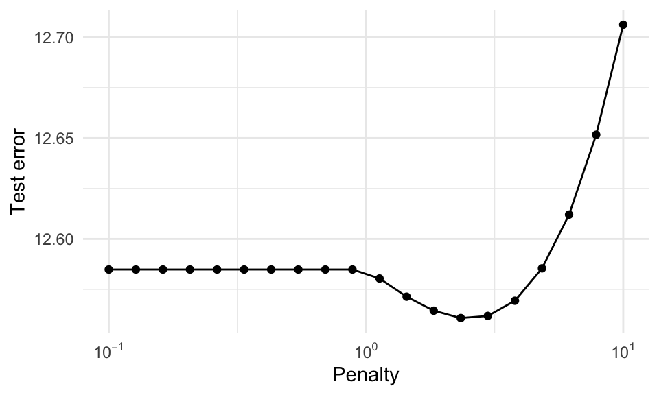
The optimal value of \(\lambda\) occurs around \(10^{-.5} \approx 3.16\). We add that parameter value to our workflow using select_best() and finalize_workflow().
best_lambda <- select_best(
  tune_results,
  metric = "rmse"
  )
best_lambda # a tibble
# A tibble: 1 × 2
penalty .config
<dbl> <chr>
1 2.34 pre0_mod14_post0my_wf_final <- my_wf |>
finalize_workflow(best_lambda)
my_wf_final══ Workflow ════════════════════════════════════════════════════════════════════
Preprocessor: Recipe
Model: linear_reg()
── Preprocessor ────────────────────────────────────────────────────────────────
3 Recipe Steps
• step_zv()
• step_dummy()
• step_normalize()
── Model ───────────────────────────────────────────────────────────────────────
Linear Regression Model Specification (regression)
Main Arguments:
penalty = 2.33572146909012
mixture = 0
Computational engine: glmnet We’re finally ready to fit the model using training data.
my_wf_fit <- my_wf_final |>
  fit(data = train)

tidy(my_wf_fit) # attractive results
Attaching package: 'Matrix'The following objects are masked from 'package:tidyr':
expand, pack, unpackLoaded glmnet 5.0# A tibble: 18 × 3
term estimate penalty
<chr> <dbl> <dbl>
1 (Intercept) 65.3 2.34
2 Apps 1.78 2.34
3 Accept 0.595 2.34
4 Enroll 0.487 2.34
5 Top10perc 2.07 2.34
6 Top25perc 1.44 2.34
7 F.Undergrad -0.464 2.34
8 P.Undergrad -2.31 2.34
9 Outstate 3.33 2.34
10 Room.Board 2.20 2.34
11 Books -0.387 2.34
12 Personal -1.27 2.34
13 PhD 1.15 2.34
14 Terminal -0.337 2.34
15 S.F.Ratio 0.746 2.34
16 perc.alumni 3.51 2.34
17 Expend -1.00 2.34
18 Private_Yes 1.40 2.34Finally, we can check the performance of our model using the test set.
results <- augment(my_wf_fit, new_data = test)
glimpse(results) # the test test plus model predictions
Rows: 195
Columns: 19
$ .pred <dbl> 72.36819, 57.01236, 81.67487, 66.47180, 76.88495, 63.56072…
$ Private <fct> Yes, Yes, Yes, Yes, Yes, Yes, No, No, Yes, Yes, No, Yes, Y…
$ Apps <dbl> 1038, 582, 2652, 1179, 1267, 619, 12809, 1734, 1879, 2496,…
$ Accept <dbl> 839, 498, 1900, 780, 1080, 516, 10308, 1729, 1658, 1402, 8…
$ Enroll <dbl> 227, 172, 484, 290, 385, 219, 3761, 951, 497, 531, 546, 48…
$ Top10perc <dbl> 30, 21, 44, 38, 44, 20, 24, 12, 36, 53, 12, 37, 11, 15, 20…
$ Top25perc <dbl> 63, 44, 77, 64, 73, 51, 49, 52, 69, 95, 36, 68, 28, 55, 50…
$ F.Undergrad <dbl> 973, 799, 1707, 1130, 1306, 1251, 22593, 3602, 1950, 2121,…
$ P.Undergrad <dbl> 306, 78, 44, 638, 28, 767, 7585, 939, 38, 69, 824, 49, 74,…
$ Outstate <dbl> 15595, 10468, 17080, 9690, 12572, 11208, 7434, 3460, 13353…
$ Room.Board <dbl> 4400, 3380, 4440, 4785, 4552, 4124, 4850, 2650, 4173, 8124…
$ Books <dbl> 300, 660, 400, 600, 400, 350, 700, 450, 540, 600, 660, 350…
$ Personal <dbl> 500, 1800, 600, 1000, 400, 1615, 2100, 1000, 821, 850, 180…
$ PhD <dbl> 79, 40, 73, 60, 79, 55, 88, 57, 78, 83, 57, 80, 63, 66, 76…
$ Terminal <dbl> 84, 41, 91, 84, 87, 65, 93, 60, 83, 93, 62, 80, 63, 68, 71…
$ S.F.Ratio <dbl> 11.3, 11.5, 9.9, 13.3, 15.3, 12.7, 18.9, 19.6, 12.7, 10.3,…
$ perc.alumni <dbl> 23, 15, 41, 21, 32, 25, 5, 5, 40, 33, 16, 17, 13, 19, 19, …
$ Expend <dbl> 11644, 8991, 11711, 7940, 9305, 6584, 4602, 4739, 9220, 12…
$ Grad.Rate <dbl> 80, 52, 76, 74, 68, 65, 48, 48, 71, 91, 46, 63, 35, 75, 58…rmse(results,
truth = Grad.Rate,
estimate = .pred) # compare predictions with observations# A tibble: 1 × 3
.metric .estimator .estimate
<chr> <chr> <dbl>
1 rmse standard 13.6This result is a slight improvement over simple linear regression.
Want to watch me explain all this? I’ve got you covered: